|
. |
Turbulence Profiling in the Canaries Observatories
.
Introduction
Although the importance of the experimental knowledge of the vertical structure of the turbulence with good statistical coverage is obvious, has been no an effort continued and systematic of these measures in the observatories, as it has happened to the seeing size. The common monitoring parameters for the turbulence characterization are insufficient for forthcoming MCAO (Multi-Conjugate Adaptive Optics) systems and large telescopes. Site quality traditionally has been characterised by seeing size (zero moment of Cn2), the stability of weather conditions, and useful observing time. Numerous publications give statistical results for sites (e.g. Vernin & Muñoz-Tuñón, 1994 and 1995) such as the Roque de los Muchachos Observatory (ORM, La Palma, Spain). On the other hand, generalized-SCIDAR is perhaps the most contrasted, extended and reliable technique. The reason, probably, is in the absence of an instrument with category of common-user providing profiles of turbulence and wind with quite high height resolution.
Vernin & Roddier (1973) proposed the classical SCIDAR (Scintillation Detection And Ranging) technique, which was developed over a period of several years (Rocca, A., Roddier, F. & Vernin, J., 1974). But this did not allow measuring the turbulence in the lower atmospheric layers above the telescope dome. In order to overcome this shortcoming, Funchs, Tallon, & Vernin (1994 and 1998) proposed the generalized-SCIDAR technique, which has been successfully tested and exploited over the last decade (Ávila, Vernin & Masciadri 1997; Ávila, Vernin & Cuevas 1998; Kluckers et al. 1998). We have developed a new instrument (Fuensalida et al, 2004; Hoegemann et al, 2004), which we call cute-SCIDAR. It is permanently installed at 1m Jacobus Kapteyn Telescope (ORM) and is based on the original generalized-SCIDAR used by the Vernin’s group of Laboratoire Universitaire d’Astrophysique de Nice (LUAN). Recently, we have developed a new version, which has been installed in Paranal Observatory.
.
Observations in ORM (2004, 2005)
In order to avoid biased statistical data, we have established to get the measurements in the period of dark nights (around new moon nights) each month. Of this way, besides fixing the statistical sample criterion, we facilitated the SCIDAR observations reducing the background emission. The programming for 2004 was the monitoring throughout one week (dark nights) every month, however technical troubles, bad weather (climatologic conditions out the limits), or overload of work of the team have made to fluctuate the sample. Because the decrease of human resources in the course of 2005, we was reduced to doing less observing nights each month. All resulting profiles were concerned about the statistical calculations, this is, no profile was rejected after data processing.
In the table 1, we resume the statistical coverage of the observations with the number of nights and the profiles each month during 2004 and 2005. We started the measurements with cute-SCIDAR instrument in the JKT on February 2004. During 2004, the average number of profiles per month was 5529 corresponding to more than 997 profiles per night each month (see last row). The total number of nights with measurements was 61 distributed throughout 11 months (5.55 nights/month). In the case of 2005, the average number of profiles per night was 903 in 43 nights throughout 12 months (3.58 nights/month).
.
|
|
Table 1.- Monthly statistical coverage of the observations during 2004 and 2005. We show the number of nights and profiles. Also, we indicate the number of profiles per night and the annual averages. |
|
. |
2004 |
2005 |
. |
Nights |
Profiles |
Nights |
Profiles |
Jan |
. |
. |
7 |
10345 |
Feb |
3 |
2322 |
1 |
380 |
Mar |
6 |
5942 |
3 |
1029 |
Apr |
8 |
9586 |
4 |
4450 |
May |
6 |
5343 |
4 |
4029 |
Jun |
5 |
5045 |
7 |
5116 |
Jul |
7 |
7530 |
4 |
4313 |
Ago |
7 |
8264 |
3 |
1337 |
Sep |
9 |
8867 |
3 |
1723 |
Oct |
2 |
1260 |
3 |
2715 |
Nov |
4 |
3847 |
2 |
1270 |
Dec |
4 |
2813 |
2 |
2123 |
TOTAL |
61 |
60819 |
43 |
38830 |
Average |
5.55 |
5529.00 |
3.58 |
3235.83 |
|
.
Global Statistics in JKT
From the individual profiles, we have computed the global statistics of the seeing size. In the figure 1a, we show the monthly median of the whole seeing, while in the figures 1b and 1c are the monthly mean of the seeing in the boundary layer (first km above ground) and the free atmosphere respectively (the bars are the standard deviation). The black circles are results belonging to 2004, and the white squares are of the 2005.
As it has been mentioned previously, all data reported here have been taken with the JKT, so that, some local effect in the surface seeing could be affected. Global statistics of the seeing on the ORM obtained from long campaigns with DIMMs (Differential Image Motion Monitors), and reported in several publications (e.g. Muñoz-Tuñón, Vernin & Varela 1997; Wilson et al. 1999; Muñoz-Tuñón 2002; Muñoz-Tuñón, Varela & Mahoney 1998, and references therein) give the typical overall seeing value for the ORM of 0.68 arc-sec and typical median of 0.64 arc-sec (available to the community in databases [ http://www.otri.iac.es/sitesting/]).
Although it makes clear a seasonal behaviour, as it is well known from DIMM (Differential Image Motion Monitor) data taken during years (Vernin & Muñoz-Tuñón, 1994 and 1995), evident differences are shown between the data of 2004 and 2005. The whole seeing goes better in the summer and get worse during the winter. The clearer discrepancies between the data of both years are during the spring. Although the tendency of the whole seeing is to have larger values during spring and summer of 2005 (except August), the largest difference is in spring, especially in May (see figure 1a).
Looking through the figures 1b and 1c, it seems clear that the differences of the whole seeing size come from the turbulence in the boundary layer. Effectively, the figure 1a shows a similar behaviour to the figure 1b, which is the variation of the seeing in the boundary layer. On the other hand, the contribution of the seeing in the free atmosphere (figure 1c) is quite similar, within the error bars, during both years. So that, as the seasonal variations as the discrepancies between years, come mainly from the turbulence produced in the first km above ground.
.
Statistics of Profiles in JKT
In the figures 2 and 3, we present the monthly average profiles of 2004 and 2005, respectively. They have been calculated from all individual profiles in each month. The systematic measurements with cute-SCIDAR instrument in JKT began on February 2004, therefore the graph of January 2004 is not shown. The X axis is the logarithmical scale of the Cn2 in unit of m-2/3 (the range goes from 10E-20 to 10E-14 m-2/3), and the Y axis is the height in km above the sea level. The horizontal line indicates the observatory height (2400 m).
A consistent layer of turbulence during the summer of 2004 is relevant around the 5 km height (see the figure 2). This characteristic appears in July and goes on until September changing the shape. It contributes to the value of the seeing in the free atmosphere, so that the improvement of the seeing in the boundary layer during the summer can not be attributed to this effect. Furthermore, another lower layer seems to be in winter and spring, which is generally unresolved around 3.5-4 km height. It could indicate a dynamic between winter and summer, by which a lower and weaker layer in winter moving upward and strengthening in summer in a range around a height of 5 km. On the other hand, when the characteristic of 5 km is present the average profile reveals a decreasing of the turbulence in a wide interval around 10 km (see July 2004). It produces a relative maximum in the surroundings of 16 km.
.
|
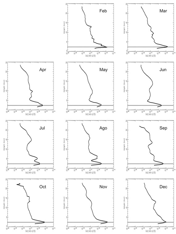 Fig. 2 .- Average profiles of Cn2 at each month of 2004. Each value is the mean of all data to its height. The systematic measurements with cute-SCIDAR instrument in JKT began on February 2004. The vertical axis is the height above the sea level in km. The horizontal lines indicate the observatory height (2.4 km). The X axis is the logarithmical scale of the Cn2 in unit of m-2/3 (the range goes from 10E-20 to 10E-14 m-2/3).
 |
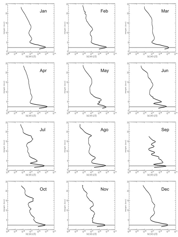 Fig. 3 .- Average profiles of Cn2 at each month of 2005. Each value is the mean of all data to its height. The vertical axis is the height above the sea level in km. The horizontal lines indicate the observatory height (2.4 km). The X axis is the logarithmical scale of the Cn2 in unit of m-2/3 (the range goes from 10E-20 to 10E-14 m-2/3)
 |
|
.
In the profiles of 2005 (Fig. 3), the characteristics are similar, although with temporal displacements. For example, the characteristic of 5 km, present in the summer of 2004, appears in May in the data of 2005, which is extended until the end of the summer (September shows a strange profile and its error bar in Fig. 1c is perceptibly large, what reveals erratic changes among those nights). It is two months ahead of 2004 and provokes an increase of the seeing in the free atmosphere on those months (May and June), unlike the remaining months in which the free atmosphere seeing becomes even smaller (Fig. 1c). As in 2004, when the 5 km layer comes out, a wide depression around 10 km and a relative maximum roughly 16 km appear: this smooth maximum becomes in a clear layer in July, and August shows a thin and weaker peak at 18 km (this higher altitude could be related to the fact that the 5 km layer is also going upward until rather 7 km). Furthermore, October has a high layer quite similar to July, although a little lower and thinner (October 2004 also shows a small trace in the same altitude). Apparently, this high layer tends to remain in autumn, which should be confirmed with more data. By another part, between April and August, the boundary layer seeing (Fig. 1b) is unusually large concerning the same period of 2004. So that, some turbulence layer remained near the ground during this period. |
| |
|
.CONTENTS:
Turbulence Profiling in the Canaries Observatories
- Introduction. Importance about the knowledge of the turbulence profiles.
- Observations in ORM and Reduction of data
- Global statistics
- Statistics of profiles in JKT (ORM)
|
|

Fig. 1.- Global statistics of the seeing size derived from the profiles. The black circles are 2004 and the white squares are 2005. a) The median of the whole seeing. b) The mean of the seeing in the boundary layer (the bars indicate the standard deviation). c) The mean of the seeing in free atmosphere.
|
|
|
|
| |
|